Virtual displacement

One degree of freedom.

Two degrees of freedom.

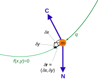
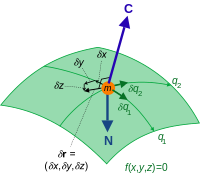
Constraint force C and virtual displacement δr for a particle of mass m confined to a curve. The resultant non-constraint force is N. The components of virtual displacement are related by a constraint equation.

In analytical mechanics, a branch of applied mathematics and physics, a virtual displacement (or infinitesimal variation) ${\displaystyle \delta \gamma }$ shows how the mechanical system's trajectory can hypothetically (hence the term virtual) deviate very slightly from the actual trajectory ${\displaystyle \gamma }$ of the system without violating the system's constraints.^{[1][2][3]: 263} For every time instant ${\displaystyle t,}$ ${\displaystyle \delta \gamma (t)}$ is a vector tangential to the configuration space at the point ${\displaystyle \gamma (t).}$ The vectors ${\displaystyle \delta \gamma (t)}$ show the directions in which ${\displaystyle \gamma (t)}$ can "go" without breaking the constraints.

For example, the virtual displacements of the system consisting of a single particle on a two-dimensional surface fill up the entire tangent plane, assuming there are no additional constraints.

If, however, the constraints require that all the trajectories ${\displaystyle \gamma }$ pass through the given point ${\displaystyle \mathbf {q} }$ at the given time ${\displaystyle \tau ,}$ i.e. ${\displaystyle \gamma (\tau )=\mathbf {q} ,}$ then ${\displaystyle \delta \gamma (\tau )=0.}$

Notations

Let ${\displaystyle M}$ be the configuration space of the mechanical system, ${\displaystyle t_{0},t_{1}\in \mathbb {R} }$ be time instants, ${\displaystyle q_{0},q_{1}\in M,}$ ${\displaystyle C^{\infty }[t_{0},t_{1}]}$ consists of smooth functions on ${\displaystyle [t_{0},t_{1}]}$, and

${\displaystyle P(M)=\{\gamma \in C^{\infty }([t_{0},t_{1}],M)\mid \gamma (t_{0})=q_{0},\ \gamma (t_{1})=q_{1}\}.}$

The constraints ${\displaystyle \gamma (t_{0})=q_{0},}$ ${\displaystyle \gamma (t_{1})=q_{1}}$ are here for illustration only. In practice, for each individual system, an individual set of constraints is required.

Definition

For each path ${\displaystyle \gamma \in P(M)}$ and ${\displaystyle \epsilon _{0}>0,}$ a variation of ${\displaystyle \gamma }$ is a function ${\displaystyle \Gamma :[t_{0},t_{1}]\times [-\epsilon _{0},\epsilon _{0}]\to M}$ such that, for every ${\displaystyle \epsilon \in [-\epsilon _{0},\epsilon _{0}],}$ ${\displaystyle \Gamma (\cdot ,\epsilon )\in P(M)}$ and ${\displaystyle \Gamma (t,0)=\gamma (t).}$ The virtual displacement ${\displaystyle \delta \gamma :[t_{0},t_{1}]\to TM}$ ${\displaystyle (TM}$ being the tangent bundle of ${\displaystyle M)}$ corresponding to the variation ${\displaystyle \Gamma }$ assigns^[1] to every ${\displaystyle t\in [t_{0},t_{1}]}$ the tangent vector

${\displaystyle \delta \gamma (t)={\frac {d\Gamma (t,\epsilon )}{d\epsilon }}{\Biggl |}_{\epsilon =0}\in T_{\gamma (t)}M.}$

In terms of the tangent map,

${\displaystyle \delta \gamma (t)=\Gamma _{*}^{t}\left({\frac {d}{d\epsilon }}{\Biggl |}_{\epsilon =0}\right).}$

Here ${\displaystyle \Gamma _{*}^{t}:T_{0}[-\epsilon ,\epsilon ]\to T_{\Gamma (t,0)}M=T_{\gamma (t)}M}$ is the tangent map of ${\displaystyle \Gamma ^{t}:[-\epsilon ,\epsilon ]\to M,}$ where ${\displaystyle \Gamma ^{t}(\epsilon )=\Gamma (t,\epsilon ),}$ and ${\displaystyle \textstyle {\frac {d}{d\epsilon }}{\Bigl |}_{\epsilon =0}\in T_{0}[-\epsilon ,\epsilon ].}$

Properties

• Coordinate representation. If ${\displaystyle \{q_{i}\}_{i=1}^{n}}$ are the coordinates in an arbitrary chart on ${\displaystyle M}$ and ${\displaystyle n=\mathop {\rm {dim}} M,}$ then

${\displaystyle \delta \gamma (t)=\sum _{i=1}^{n}{\frac {d[q_{i}(\Gamma (t,\epsilon ))]}{d\epsilon }}{\Biggl |}_{\epsilon =0}\cdot {\frac {d}{dq_{i}}}{\Biggl |}_{\gamma (t)}.}$

• If, for some time instant ${\displaystyle \tau }$ and every ${\displaystyle \gamma \in P(M),}$ ${\displaystyle \gamma (\tau )={\text{const}},}$ then, for every ${\displaystyle \gamma \in P(M),}$ ${\displaystyle \delta \gamma (\tau )=0.}$

• If ${\displaystyle \textstyle \gamma ,{\frac {d\gamma }{dt}}\in P(M),}$ then ${\displaystyle \delta {\frac {d\gamma }{dt}}={\frac {d}{dt}}\delta \gamma .}$

Examples

Free particle in R³

A single particle freely moving in ${\displaystyle \mathbb {R} ^{3}}$ has 3 degrees of freedom. The configuration space is ${\displaystyle M=\mathbb {R} ^{3},}$ and ${\displaystyle P(M)=C^{\infty }([t_{0},t_{1}],M).}$ For every path ${\displaystyle \gamma \in P(M)}$ and a variation ${\displaystyle \Gamma (t,\epsilon )}$ of ${\displaystyle \gamma ,}$ there exists a unique ${\displaystyle \sigma \in T_{0}\mathbb {R} ^{3}}$ such that ${\displaystyle \Gamma (t,\epsilon )=\gamma (t)+\sigma (t)\epsilon +o(\epsilon ),}$ as ${\displaystyle \epsilon \to 0.}$ By the definition,

${\displaystyle \delta \gamma (t)=\left({\frac {d}{d\epsilon }}{\Bigl (}\gamma (t)+\sigma (t)\epsilon +o(\epsilon ){\Bigr )}\right){\Biggl |}_{\epsilon =0}}$

which leads to

${\displaystyle \delta \gamma (t)=\sigma (t)\in T_{\gamma (t)}\mathbb {R} ^{3}.}$

Free particles on a surface

${\displaystyle N}$ particles moving freely on a two-dimensional surface ${\displaystyle S\subset \mathbb {R} ^{3}}$ have ${\displaystyle 2N}$ degree of freedom. The configuration space here is

${\displaystyle M=\{(\mathbf {r} _{1},\ldots ,\mathbf {r} _{N})\in \mathbb {R} ^{3\,N}\mid \mathbf {r} _{i}\in \mathbb {R} ^{3};\ \mathbf {r} _{i}\neq \mathbf {r} _{j}\ {\text{if}}\ i\neq j\},}$

where ${\displaystyle \mathbf {r} _{i}\in \mathbb {R} ^{3}}$ is the radius vector of the ${\displaystyle i^{\text{th}}}$ particle. It follows that

${\displaystyle T_{(\mathbf {r} _{1},\ldots ,\mathbf {r} _{N})}M=T_{\mathbf {r} _{1}}S\oplus \ldots \oplus T_{\mathbf {r} _{N}}S,}$

and every path ${\displaystyle \gamma \in P(M)}$ may be described using the radius vectors ${\displaystyle \mathbf {r} _{i}}$ of each individual particle, i.e.

${\displaystyle \gamma (t)=(\mathbf {r} _{1}(t),\ldots ,\mathbf {r} _{N}(t)).}$

This implies that, for every ${\displaystyle \delta \gamma (t)\in T_{(\mathbf {r} _{1}(t),\ldots ,\mathbf {r} _{N}(t))}M,}$

${\displaystyle \delta \gamma (t)=\delta \mathbf {r} _{1}(t)\oplus \ldots \oplus \delta \mathbf {r} _{N}(t),}$

where ${\displaystyle \delta \mathbf {r} _{i}(t)\in T_{\mathbf {r} _{i}(t)}S.}$ Some authors express this as

${\displaystyle \delta \gamma =(\delta \mathbf {r} _{1},\ldots ,\delta \mathbf {r} _{N}).}$

Rigid body rotating around fixed point

A rigid body rotating around a fixed point with no additional constraints has 3 degrees of freedom. The configuration space here is ${\displaystyle M=SO(3),}$ the special orthogonal group of dimension 3 (otherwise known as 3D rotation group), and ${\displaystyle P(M)=C^{\infty }([t_{0},t_{1}],M).}$ We use the standard notation ${\displaystyle {\mathfrak {so}}(3)}$ to refer to the three-dimensional linear space of all skew-symmetric three-dimensional matrices. The exponential map ${\displaystyle \exp :{\mathfrak {so}}(3)\to SO(3)}$ guarantees the existence of ${\displaystyle \epsilon _{0}>0}$ such that, for every path ${\displaystyle \gamma \in P(M),}$ its variation ${\displaystyle \Gamma (t,\epsilon ),}$ and ${\displaystyle t\in [t_{0},t_{1}],}$ there is a unique path ${\displaystyle \Theta ^{t}\in C^{\infty }([-\epsilon _{0},\epsilon _{0}],{\mathfrak {so}}(3))}$ such that ${\displaystyle \Theta ^{t}(0)=0}$ and, for every ${\displaystyle \epsilon \in [-\epsilon _{0},\epsilon _{0}],}$ ${\displaystyle \Gamma (t,\epsilon )=\gamma (t)\exp(\Theta ^{t}(\epsilon )).}$ By the definition,

${\displaystyle \delta \gamma (t)=\left({\frac {d}{d\epsilon }}{\Bigl (}\gamma (t)\exp(\Theta ^{t}(\epsilon )){\Bigr )}\right){\Biggl |}_{\epsilon =0}=\gamma (t){\frac {d\Theta ^{t}(\epsilon )}{d\epsilon }}{\Biggl |}_{\epsilon =0}.}$

Since, for some function ${\displaystyle \sigma :[t_{0},t_{1}]\to {\mathfrak {so}}(3),}$ ${\displaystyle \Theta ^{t}(\epsilon )=\epsilon \sigma (t)+o(\epsilon )}$, as ${\displaystyle \epsilon \to 0}$,

${\displaystyle \delta \gamma (t)=\gamma (t)\sigma (t)\in T_{\gamma (t)}SO(3).}$

See also

• D'Alembert principle
• Virtual work

References

- ^ a b Takhtajan, Leon A. (2017). "Part 1. Classical Mechanics". Classical Field Theory (PDF). Department of Mathematics, Stony Brook University, Stony Brook, NY.
- ^ Goldstein, H.; Poole, C. P.; Safko, J. L. (2001). Classical Mechanics (3rd ed.). Addison-Wesley. p. 16. ISBN 978-0-201-65702-9.
- ^ Torby, Bruce (1984). "Energy Methods". Advanced Dynamics for Engineers. HRW Series in Mechanical Engineering. United States of America: CBS College Publishing. ISBN 0-03-063366-4.