Sign function

In mathematics, the sign function or signum function (from signum, Latin for "sign") is a function that has the value −1, +1 or 0 according to whether the sign of a given real number is positive or negative, or the given number is itself zero. In mathematical notation the sign function is often represented as ${\displaystyle \operatorname {sgn} x}$ or ${\displaystyle \operatorname {sgn}(x)}$.^[1]

Definition

The signum function of a real number ${\displaystyle x}$ is a piecewise function which is defined as follows:^[1]

The law of trichotomy states that every real number must be positive, negative or zero. The signum function denotes which unique category a number falls into by mapping it to one of the values −1, +1 or 0, which can then be used in mathematical expressions or further calculations.

For example:

Basic properties

Any real number can be expressed as the product of its absolute value and its sign function:

It follows that whenever ${\displaystyle x}$ is not equal to 0 we have

Similarly, for any real number ${\displaystyle x}$,

We can also be certain that: and so

Some algebraic identities

The signum can also be written using the Iverson bracket notation:

The signum can also be written using the floor and the absolute value functions:

The signum function has a very simple definition if ${\displaystyle 0^{0}}$ is accepted to be equal to 1. Then signum can be written for all real numbers as

Properties in mathematical analysis

Discontinuity at zero

Although the sign function takes the value −1 when ${\displaystyle x}$ is negative, the ringed point (0, −1) in the plot of ${\displaystyle \operatorname {sgn} x}$ indicates that this is not the case when ${\displaystyle x=0}$. Instead, the value jumps abruptly to the solid point at (0, 0) where ${\displaystyle \operatorname {sgn}(0)=0}$. There is then a similar jump to ${\displaystyle \operatorname {sgn}(x)=+1}$ when ${\displaystyle x}$ is positive. Either jump demonstrates visually that the sign function ${\displaystyle \operatorname {sgn} x}$ is discontinuous at zero, even though it is continuous at any point where ${\displaystyle x}$ is either positive or negative.

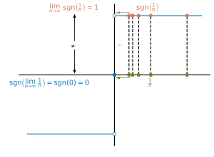
These observations are confirmed by any of the various equivalent formal definitions of continuity in mathematical analysis. A function ${\displaystyle f(x)}$, such as ${\displaystyle \operatorname {sgn}(x),}$ is continuous at a point ${\displaystyle x=a}$ if the value ${\displaystyle f(a)}$ can be approximated arbitrarily closely by the sequence of values ${\displaystyle f(a_{1}),f(a_{2}),f(a_{3}),\dots ,}$ where the ${\displaystyle a_{n}}$ make up any infinite sequence which becomes arbitrarily close to ${\displaystyle a}$ as ${\displaystyle n}$ becomes sufficiently large. In the notation of mathematical limits, continuity of ${\displaystyle f}$ at ${\displaystyle a}$ requires that ${\displaystyle f(a_{n})\to f(a)}$ as ${\displaystyle n\to \infty }$ for any sequence ${\displaystyle \left(a_{n}\right)_{n=1}^{\infty }}$ for which ${\displaystyle a_{n}\to a.}$ The arrow symbol can be read to mean approaches, or tends to, and it applies to the sequence as a whole.

This criterion fails for the sign function at ${\displaystyle a=0}$. For example, we can choose ${\displaystyle a_{n}}$ to be the sequence ${\displaystyle 1,{\tfrac {1}{2}},{\tfrac {1}{3}},{\tfrac {1}{4}},\dots ,}$ which tends towards zero as ${\displaystyle n}$ increases towards infinity. In this case, ${\displaystyle a_{n}\to a}$ as required, but ${\displaystyle \operatorname {sgn}(a)=0}$ and ${\displaystyle \operatorname {sgn}(a_{n})=+1}$ for each ${\displaystyle n,}$ so that ${\displaystyle \operatorname {sgn}(a_{n})\to 1\neq \operatorname {sgn}(a)}$. This counterexample confirms more formally the discontinuity of ${\displaystyle \operatorname {sgn} x}$ at zero that is visible in the plot.

Despite the sign function having a very simple form, the step change at zero causes difficulties for traditional calculus techniques, which are quite stringent in their requirements. Continuity is a frequent constraint. One solution can be to approximate the sign function by a smooth continuous function; others might involve less stringent approaches that build on classical methods to accommodate larger classes of function.

Smooth approximations and limits

The signum function coincides with the limits

and as well as,

Here, ${\displaystyle \tanh(x)}$ is the Hyperbolic tangent and the superscript of -1, above it, is shorthand notation for the inverse function of the Trigonometric function, tangent.

For ${\displaystyle k>1}$, a smooth approximation of the sign function is

Another approximation is which gets sharper as ${\displaystyle \varepsilon \to 0}$; note that this is the derivative of ${\displaystyle {\sqrt {x^{2}+\varepsilon ^{2}}}}$. This is inspired from the fact that the above is exactly equal for all nonzero ${\displaystyle x}$ if ${\displaystyle \varepsilon =0}$, and has the advantage of simple generalization to higher-dimensional analogues of the sign function (for example, the partial derivatives of ${\displaystyle {\sqrt {x^{2}+y^{2}}}}$).

See Heaviside step function § Analytic approximations.

Differentiation and integration

The signum function ${\displaystyle \operatorname {sgn} x}$ is differentiable everywhere except when ${\displaystyle x=0.}$ Its derivative is zero when ${\displaystyle x}$ is non-zero:

This follows from the differentiability of any constant function, for which the derivative is always zero on its domain of definition. The signum ${\displaystyle \operatorname {sgn} x}$ acts as a constant function when it is restricted to the negative open region ${\displaystyle x<0,}$ where it equals -1. It can similarly be regarded as a constant function within the positive open region ${\displaystyle x>0,}$ where the corresponding constant is +1. Although these are two different constant functions, their derivative is equal to zero in each case.

It is not possible to define a classical derivative at ${\displaystyle x=0}$, because there is a discontinuity there. Nevertheless, the signum function has a definite integral between any pair of finite values a and b, even when the interval of integration includes zero. The resulting integral for a and b is then equal to the difference between their absolute values:

Conversely, the signum function is the derivative of the absolute value function, except where there is an abrupt change in gradient before and after zero:

We can understand this as before by considering the definition of the absolute value ${\displaystyle |x|}$ on the separate regions ${\displaystyle x<0}$ and ${\displaystyle x<0.}$ For example, the absolute value function is identical to ${\displaystyle x}$ in the region ${\displaystyle x>0,}$ whose derivative is the constant value +1, which equals the value of ${\displaystyle \operatorname {sgn} x}$ there.

Because the absolute value is a convex function, there is at least one subderivative at every point, including at the origin. Everywhere except zero, the resulting subdifferential consists of a single value, equal to the value of the sign function. In contrast, there are many subderivatives at zero, with just one of them taking the value ${\displaystyle \operatorname {sgn}(0)=0}$. A subderivative value 0 occurs here because the absolute value function is at a minimum. The full family of valid subderivatives at zero constitutes the subdifferential interval ${\displaystyle [-1,1]}$, which might be thought of informally as "filling in" the graph of the sign function with a vertical line through the origin, making it continuous as a two dimensional curve.

In integration theory, the signum function is a weak derivative of the absolute value function. Weak derivatives are equivalent if they are equal almost everywhere, making them impervious to isolated anomalies at a single point. This includes the change in gradient of the absolute value function at zero, which prohibits there being a classical derivative.

Although it is not differentiable at ${\displaystyle x=0}$ in the ordinary sense, under the generalized notion of differentiation in distribution theory, the derivative of the signum function is two times the Dirac delta function. This can be demonstrated using the identity ^[2]

where ${\displaystyle H(x)}$ is the Heaviside step function using the standard ${\displaystyle H(0)={\frac {1}{2}}}$ formalism. Using this identity, it is easy to derive the distributional derivative:^[3]

Fourier transform

The Fourier transform of the signum function is^[4]

where ${\displaystyle PV}$ means taking the Cauchy principal value.

Generalizations

Complex signum

The signum function can be generalized to complex numbers as:

for any complex number ${\displaystyle z}$ except ${\displaystyle z=0}$. The signum of a given complex number ${\displaystyle z}$ is the point on the unit circle of the complex plane that is nearest to ${\displaystyle z}$. Then, for ${\displaystyle z\neq 0}$, where ${\displaystyle \arg }$ is the complex argument function.

For reasons of symmetry, and to keep this a proper generalization of the signum function on the reals, also in the complex domain one usually defines, for ${\displaystyle z=0}$:

Another generalization of the sign function for real and complex expressions is ${\displaystyle {\text{csgn}}}$,^[5] which is defined as:

where ${\displaystyle {\text{Re}}(z)}$ is the real part of ${\displaystyle z}$ and ${\displaystyle {\text{Im}}(z)}$ is the imaginary part of ${\displaystyle z}$.

We then have (for ${\displaystyle z\neq 0}$):

Polar decomposition of matrices

Thanks to the Polar decomposition theorem, a matrix ${\displaystyle {\boldsymbol {A}}\in \mathbb {K} ^{n\times n}}$ (${\displaystyle n\in \mathbb {N} }$ and ${\displaystyle \mathbb {K} \in \{\mathbb {R} ,\mathbb {C} \}}$) can be decomposed as a product ${\displaystyle {\boldsymbol {Q}}{\boldsymbol {P}}}$ where ${\displaystyle {\boldsymbol {Q}}}$ is a unitary matrix and ${\displaystyle {\boldsymbol {P}}}$ is a self-adjoint, or Hermitian, positive definite matrix, both in ${\displaystyle \mathbb {K} ^{n\times n}}$. If ${\displaystyle {\boldsymbol {A}}}$ is invertible then such a decomposition is unique and ${\displaystyle {\boldsymbol {Q}}}$ plays the role of ${\displaystyle {\boldsymbol {A}}}$'s signum. A dual construction is given by the decomposition ${\displaystyle {\boldsymbol {A}}={\boldsymbol {S}}{\boldsymbol {R}}}$ where ${\displaystyle {\boldsymbol {R}}}$ is unitary, but generally different than ${\displaystyle {\boldsymbol {Q}}}$. This leads to each invertible matrix having a unique left-signum ${\displaystyle {\boldsymbol {Q}}}$ and right-signum ${\displaystyle {\boldsymbol {R}}}$.

In the special case where ${\displaystyle \mathbb {K} =\mathbb {R} ,\ n=2,}$ and the (invertible) matrix ${\displaystyle {\boldsymbol {A}}=\left[{\begin{array}{rr}a&-b\\b&a\end{array}}\right]}$, which identifies with the (nonzero) complex number ${\displaystyle a+\mathrm {i} b=c}$, then the signum matrices satisfy ${\displaystyle {\boldsymbol {Q}}={\boldsymbol {P}}=\left[{\begin{array}{rr}a&-b\\b&a\end{array}}\right]/|c|}$ and identify with the complex signum of ${\displaystyle c}$, ${\displaystyle \operatorname {sgn} c=c/|c|}$. In this sense, polar decomposition generalizes to matrices the signum-modulus decomposition of complex numbers.

Signum as a generalized function

At real values of ${\displaystyle x}$, it is possible to define a generalized function–version of the signum function, ${\displaystyle \varepsilon (x)}$ such that ${\displaystyle \varepsilon (x)^{2}=1}$ everywhere, including at the point ${\displaystyle x=0}$, unlike ${\displaystyle \operatorname {sgn} }$, for which ${\displaystyle (\operatorname {sgn} 0)^{2}=0}$. This generalized signum allows construction of the algebra of generalized functions, but the price of such generalization is the loss of commutativity. In particular, the generalized signum anticommutes with the Dirac delta function^[6]

in addition, ${\displaystyle \varepsilon (x)}$ cannot be evaluated at ${\displaystyle x=0}$; and the special name, ${\displaystyle \varepsilon }$ is necessary to distinguish it from the function ${\displaystyle \operatorname {sgn} }$. (${\displaystyle \varepsilon (0)}$ is not defined, but ${\displaystyle \operatorname {sgn} 0=0}$.)

See also

• Absolute value
• Heaviside function
• Negative number
• Rectangular function
• Sigmoid function (Hard sigmoid)
• Step function (Piecewise constant function)
• Three-way comparison
• Zero crossing
• Polar decomposition

Notes